差速轮运动学模型

机器人坐标系下的变换

运动特性为两轮差速驱动，其底部后方两个同构驱动轮的转动为其提供动力，前方的随动轮起支撑作用并不推动其运动，如下图两轮差速驱动示意图所示。

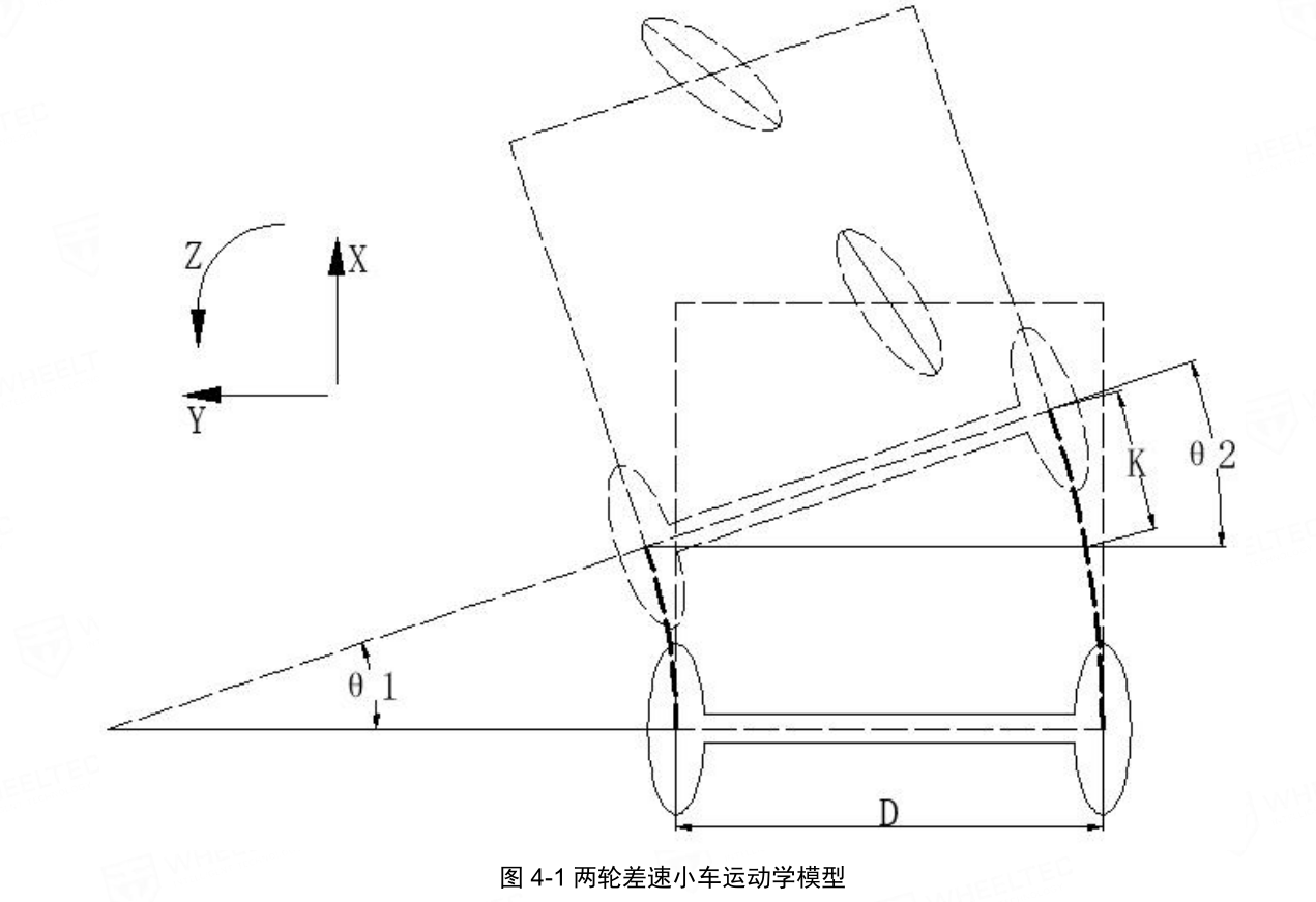
机器人的运动简化模型如图 4-1 所示，X 轴正方向为前进、Y 轴正方向为左平移、Z 轴正方向为逆时针。机器人两个轮子之间的间距为 D，机器人 X 轴和 Z 轴的速度分别为： $V_x$ 和 $V_z$ ，机器人左轮和右轮的速度分别为： $V_l$ 和 $V_r$ 。

假设机器人往一个左前的方向行进了一段距离，设机器人的右轮比左轮多走的距离近似为 K, 以机器人的轮子上的点作为参考点做延长参考线，可得： $θ_1 = θ_2$ 。由于这个 $Δ_t$ 很小，因此角度的变化量 $θ_1$ 也很小，因此有近似公式：

\theta_{2} \approx \sin \left(\theta_{2}\right)=\frac{K}{D}

由数学分析可以得到下面的式子：

\begin{equation} \mathrm{K}=\left(\mathrm{V}_{\mathrm{R}}-\mathrm{V}_{\mathrm{L}}\right) * \Delta \mathrm{t}, \quad \omega=\frac{\theta_{1}}{\Delta \mathrm{t}} \end{equation}

由上面的公式和式子可以求解出运动学正解的结果：机器人 X 轴方向速度

V_x=(V_l+V_r) / 2

机器人 Z 轴方向速度：

V_z=（V_r - V_l）/D

由正解直接反推得出运动学逆解的结果：

机器人左轮的速度：

V_l = V_x -（V_z * D）/2

机器人右轮的速度：

V_r = V_x +（V_z * D）/2

实现

运动学正解

/**
 * @brief 轮子线速度到机器人坐标速度的变换
 *        Vx = (Vl + Vr) / 2
 *        Vz = (Vr - Vl) / D
 * @return Eigen::Vector3f 机器人坐标系下的速度
 */
Eigen::Vector3f MotorToRobotSpeed(void)
{
    Eigen::Vector3f robot_speed;

    robot_speed(0) = -0.5f * motor_line_speed_measure_(0) + 0.5f * motor_line_speed_measure_(1);
    robot_speed(1) = 0 * motor_line_speed_measure_(0) + 0 * motor_line_speed_measure_(1);
    robot_speed(2) = (0.5f / body_radius_) * (motor_line_speed_measure_(0) + motor_line_speed_measure_(1));

    return robot_speed;
}

运动学逆解

/**
 * @brief 机器人坐标速度到轮子线速度的变换
 *        Vl = -Vx + (Vz * D) / 2
 *        Vr = Vx + (Vz * D) / 2
 * @param robot_speed 机器人坐标系下的速度
 * @return None
 */
void RobotToMotorSpeed(Eigen::Vector3f& robot_speed)
{
    motor_line_speed_target_(0) =  -1 * robot_speed(0)  + 0 * robot_speed(1) + body_radius_ * robot_speed(2);
    motor_line_speed_target_(1) =   1 * robot_speed(0)  + 0 * robot_speed(1) + body_radius_ * robot_speed(2);

    if(motor_num_ >= 4) {
        motor_line_speed_target_(2) = motor_line_speed_target_(0);
        motor_line_speed_target_(3) = motor_line_speed_target_(1);
    }
}

坐标系旋转

全局坐标系到机器人坐标系的变换

一个平面坐标系逆时针旋转一个角度后得到另一个坐标系，则同一个点在这两个坐标系之间的几何关系如下：

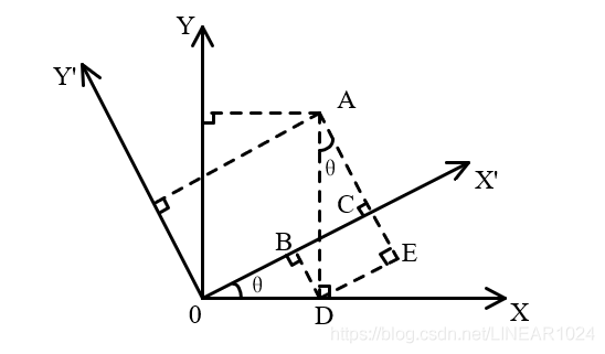
由上图可得：

\begin{equation} \begin{aligned} x^{\prime} &=O B+B C \\ &=O D \cos \theta+A D \sin \theta \\ &=x \cos \theta+y \sin \theta \end{aligned} \end{equation}

\begin{equation} \begin{aligned} y^{\prime} &=A E-C E \\ &=A D \cos \theta-O D \sin \theta \\ &=y \cos \theta-x \sin \theta \end{aligned} \end{equation}

则反过来的关系如下：

\begin{equation} \left[\begin{array}{l} x \\ y \end{array}\right]=\left[\begin{array}{cc} \cos \theta & -\sin \theta \\ \sin \theta & \cos \theta \end{array}\right]\left[\begin{array}{l} x^{\prime} \\ y^{\prime} \end{array}\right] \end{equation}

则反过来的关系如下：

\begin{equation} \left[\begin{array}{l} x \\ y \end{array}\right]=\left[\begin{array}{cc} \cos \theta & -\sin \theta \\ \sin \theta & \cos \theta \end{array}\right]\left[\begin{array}{l} x^{\prime} \\ y^{\prime} \end{array}\right] \end{equation}

实现

正解

/**
 * @brief 世界坐标到机器人坐标的速度变换
 * @param global_speed 为 Global 坐标的速度向量 xyw
 * @return Eigen::Vector3f Robot 坐标的速度向量 xyw
 */
Eigen::Vector3f GlobalToRobotSpeed(Eigen::Vector3f& global_speed)
{
    Eigen::Vector3f robot_speed;
    Eigen::Matrix3f rotate_mat;

    rotate_mat <<  cos(global_coordinat_z_), sin(global_coordinat_z_), 0.0f,
                  -sin(global_coordinat_z_), cos(global_coordinat_z_), 0.0f,
                  0.0f,                      0.0f,                     1.0f;
    robot_speed = rotate_mat * global_speed;

    return robot_speed;
}

逆解

/**
 * @brief 机器人坐标到世界坐标的速度变换
 * @param robot_speed Robot 坐标的速度向量 xyw
 * @return Eigen::Vector3f Global 坐标的速度向量 xyw
 */
Eigen::Vector3f RobotToGlobalSpeed(Eigen::Vector3f& robot_speed)
{
    Eigen::Vector3f global_speed;
    Eigen::Matrix3f rotate_mat;

    rotate_mat << cos(global_coordinat_z_), -sin(global_coordinat_z_), 0.0f,
                  sin(global_coordinat_z_),  cos(global_coordinat_z_), 0.0f,
                  0.0f,                      0.0f,                     1.0f;
    global_speed = rotate_mat * robot_speed;

    return global_speed;
}